## Creating a function: regplot
## Combine the lm, plot and abline functions to create a regression fit plot function
regplot=function(x,y){
  fit=lm(y~x)
  plot(x,y)
  abline(fit,col="red")
}EPPS 6323: Lab03 R programming (Exploratory Data Analysis)
R Programming (EDA)
attach(ISLR::Carseats)
regplot(Price,Sales)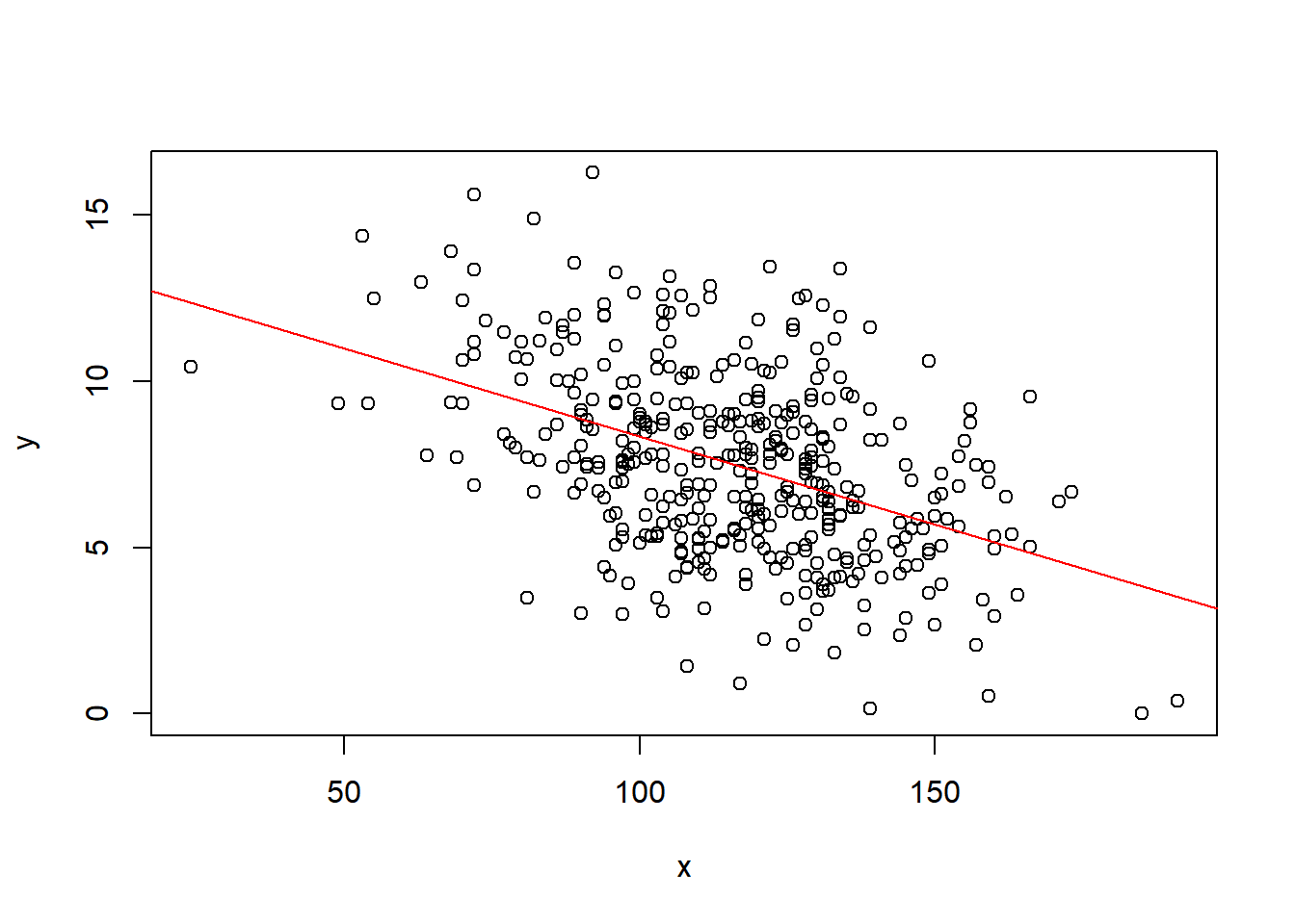
## Allow extra room for additional arguments/specifications
regplot=function(x,y,...){
  fit=lm(y~x)
  plot(x,y,...)
  abline(fit,col="red")
}  # "..." is called ellipsis, which is designed to take any number of named or unnamed arguments.
regplot(Price,Sales,xlab="Price",ylab="Sales",col="blue",pch=20)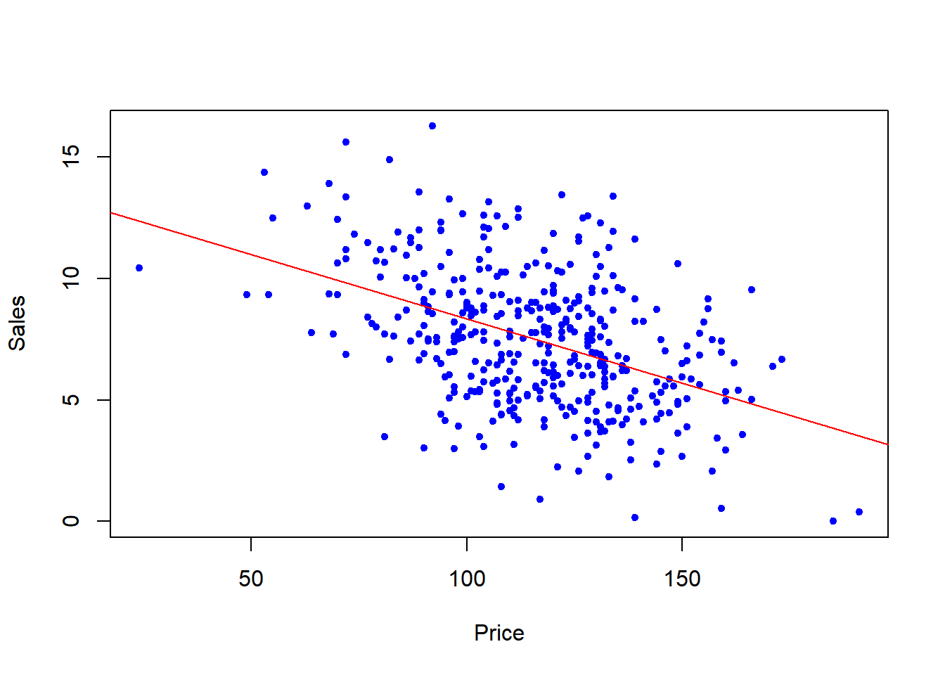
(Adapted from Stackoverflow examples) (Objectives: Use plotly, reshape packages, interactive visualization)
library(tidyverse)
library(plotly)
data(iris)
attach(iris)
# Generate plot on three quantitative variables
iris_plot <- plot_ly(iris,
                     x = Sepal.Length,
                     y = Sepal.Width,
                     z = Petal.Length,
                     type = "scatter3d",
                     mode = "markers",
                     size = 0.02)
iris_plot
# Regression object
petal_lm <- lm(Petal.Length ~ 0 + Sepal.Length + Sepal.Width,
data = iris)
library(reshape2)
#load data
petal_lm <- lm(Petal.Length ~ 0 + Sepal.Length + Sepal.Width,data = iris)
# Setting resolution parameter
graph_reso <- 0.05
#Setup Axis
axis_x <- seq(min(iris$Sepal.Length), max(iris$Sepal.Length), by = graph_reso)
axis_y <- seq(min(iris$Sepal.Width), max(iris$Sepal.Width), by = graph_reso)
# Regression surface
# Rearranging data for plotting
petal_lm_surface <- expand.grid(Sepal.Length = axis_x,Sepal.Width = axis_y,KEEP.OUT.ATTRS = F)
petal_lm_surface$Petal.Length <- predict.lm(petal_lm, newdata = petal_lm_surface)
petal_lm_surface <- acast(petal_lm_surface, Sepal.Width ~ Sepal.Length, value.var = "Petal.Length")
hcolors=c("orange","blue","green")[iris$Species]
iris_plot <- plot_ly(iris,
x = ~Sepal.Length,
y = ~Sepal.Width,
z = ~Petal.Length,
text = Species,
type = "scatter3d",
mode = "markers",
marker = list(color = hcolors),
size=0.02)
# Add surface
iris_plot <- add_trace(p = iris_plot,
z = petal_lm_surface,
x = axis_x,
y = axis_y,
type = "surface",mode = "markers",
marker = list(color = hcolors))
iris_plotRegression object
petal_lm <- lm(Petal.Length ~ 0 + Sepal.Length + Sepal.Width,
               data = iris)
summary(petal_lm)
Call:
lm(formula = Petal.Length ~ 0 + Sepal.Length + Sepal.Width, data = iris)

Residuals:
     Min       1Q   Median       3Q      Max
-1.70623 -0.51867 -0.08334  0.49844  1.93093

Coefficients:
             Estimate Std. Error t value Pr(>|t|)
Sepal.Length  1.56030    0.04557   34.24   <2e-16 ***
Sepal.Width  -1.74570    0.08709  -20.05   <2e-16 ***
---
Signif. codes:  0 '***' 0.001 '**' 0.01 '*' 0.05 '.' 0.1 ' ' 1

Residual standard error: 0.6869 on 148 degrees of freedom
Multiple R-squared:  0.973, Adjusted R-squared:  0.9726
F-statistic:  2663 on 2 and 148 DF,  p-value: < 2.2e-16