Unsupervised learning involves algorithms that detect patterns or grouping structures in data without relying on labeled information like dependent variables. Instead, it explores the inherent structure and possible groupings of unlabeled data, often used as a pre-processing step for supervised learning.
In unsupervised learning, there’s no explicit dependent variable for prediction (Y). The focus is on revealing patterns within measurements (X1, X2, …, Xp) and identifying any underlying subgroups among observations.
This section introduces two main methods:
Principal Component Analysis (PCA)
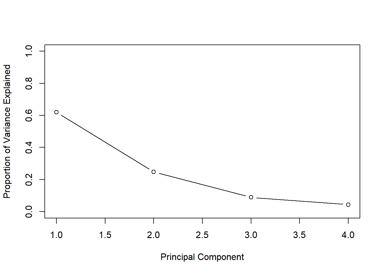
Principal Components Analysis (PCA) generates a correlated, low-dimensional representation of a dataset by identifying linear combinations of variables with maximal variance and mutually uncorrelated.
The first principal component of a set of features \((X_1, X_2, . . . , X_p)\) is the normalized linear combination of the features: \[ Z_1 = \phi_{11}X_1 +\phi_{21}X_2 +...+\phi_{p1}X_p \] ,
which has the largest variance.
“Normalized” means that: \(\sum_{j=1}^p\phi_{j1}^2 = 1\).
The elements \((\phi_{11}, . . . , \phi_{p1})\) is the loading of the first principal component.
The loadings, collectively, make up the principal compobebt loading “vector” = \(\phi_1= (\phi_{11} \phi_{21} ... \phi_{p1})^T\)
We constrain the loadings to set the sum of squares = 1. Otherwise, setting these elements to be arbitrarily large in absolute value might result in an arbitrarily large variance.
Clustering
K-Means Clustering
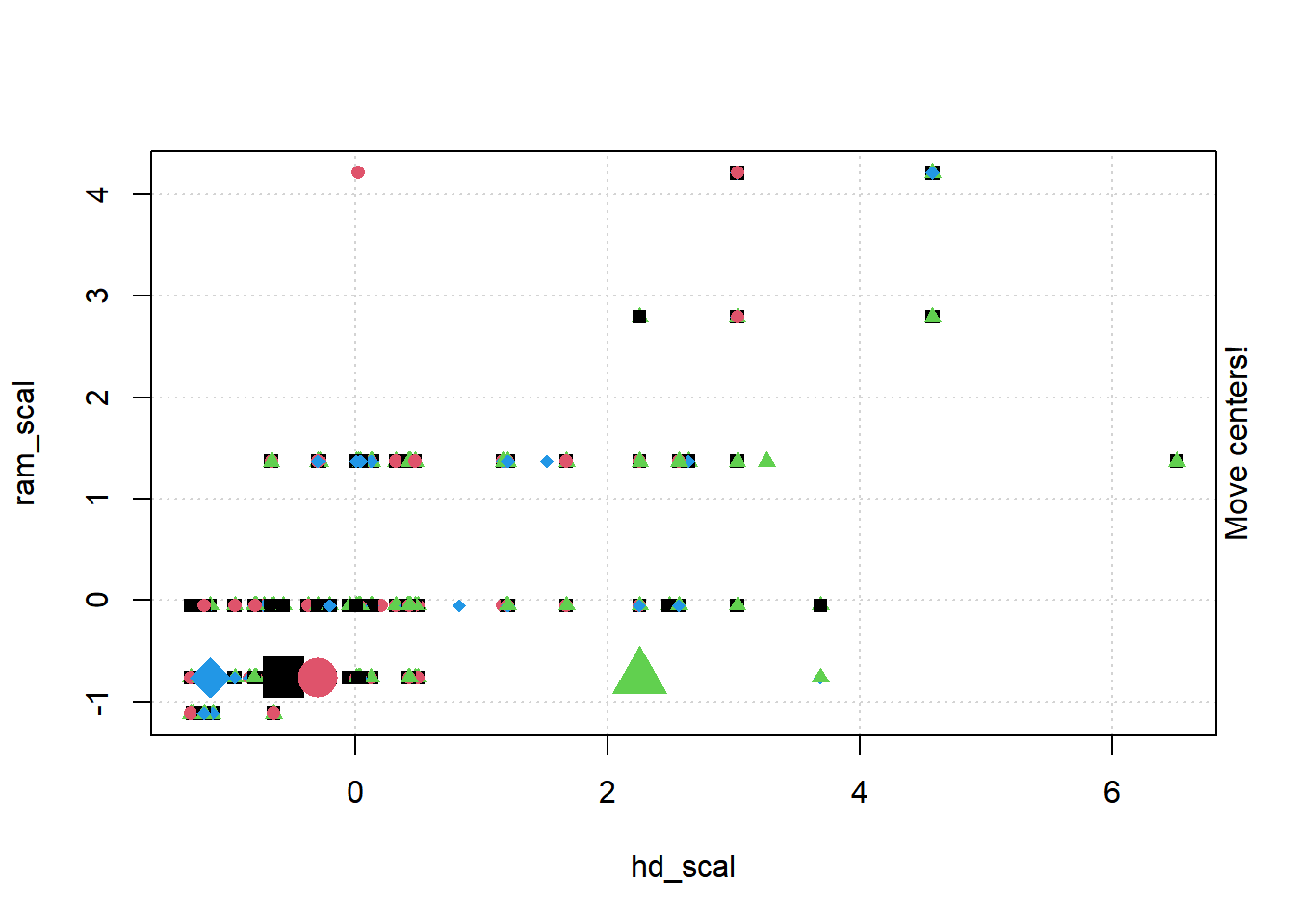
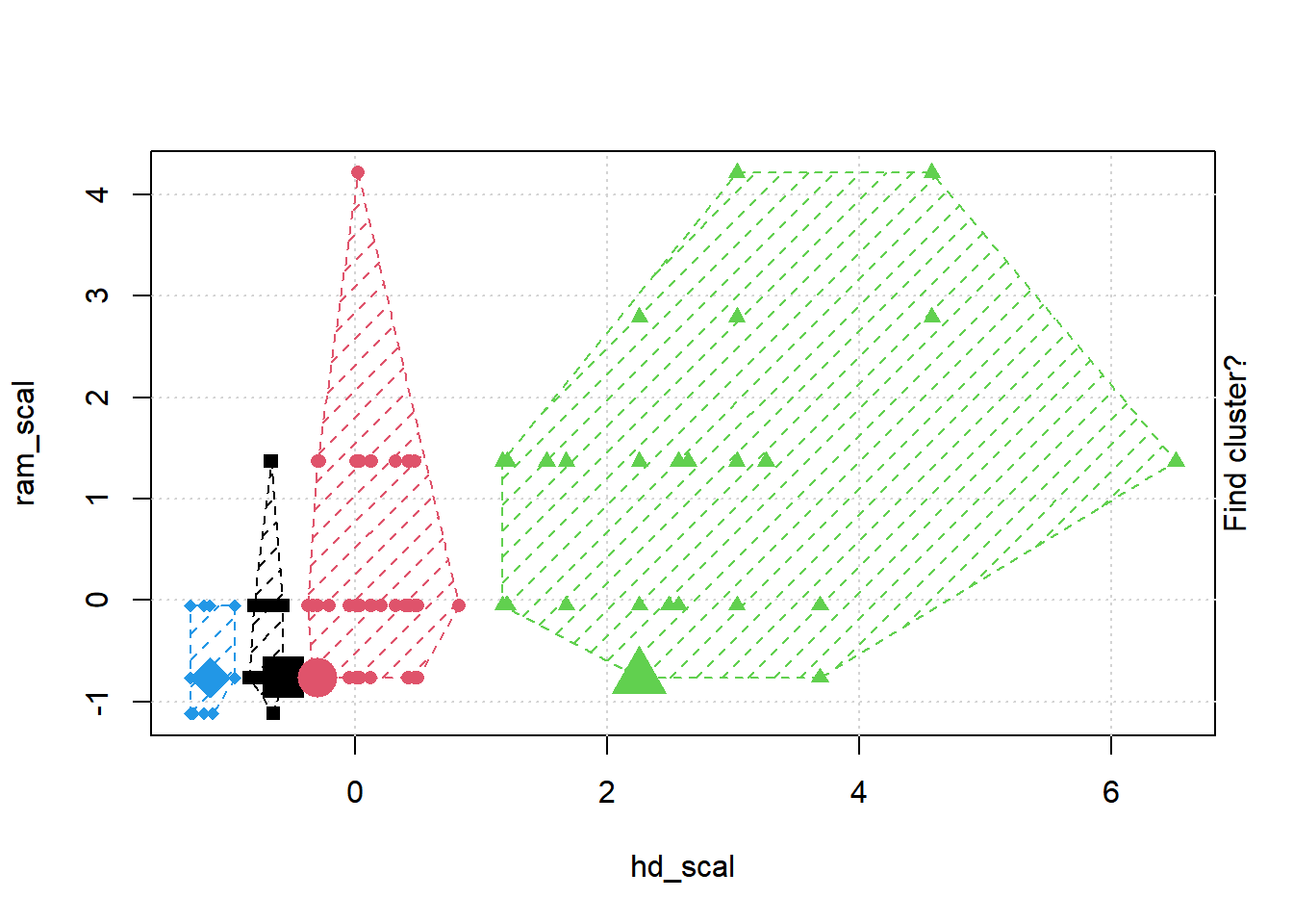
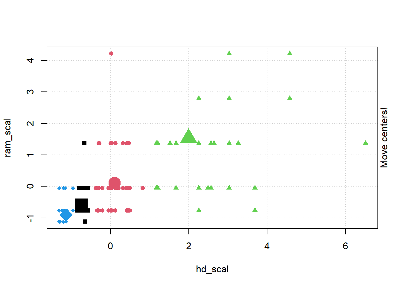
K-Means Clustering is a method used to divide data points into K groups while minimizing the sum of squares from each point to its assigned cluster center within each group.
Hierarchical Clustering
Hierarchical clustering offers an alternative approach that doesn’t require a pre-determined or pre-specified or a particular value/choice of \((K)\).
One advantage of Hierarchical Clustering is its ability to generate a dendrogram - a tree-based depiction of observations.
The dendrogram is constructed by merging clusters from the leaves to the trunk. It provides a visual representation of data relationships, allowing for subgroup identification by cutting the dendrogram at desired similarity levels.
Practice Workshop: Principal Component Analysis and Clustering Methods
1. Principal Component Analysis (PCA)
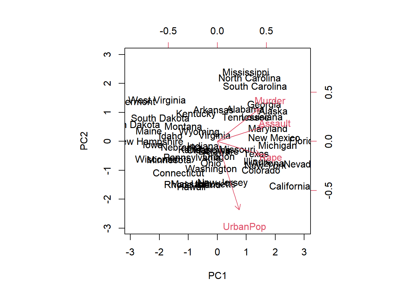
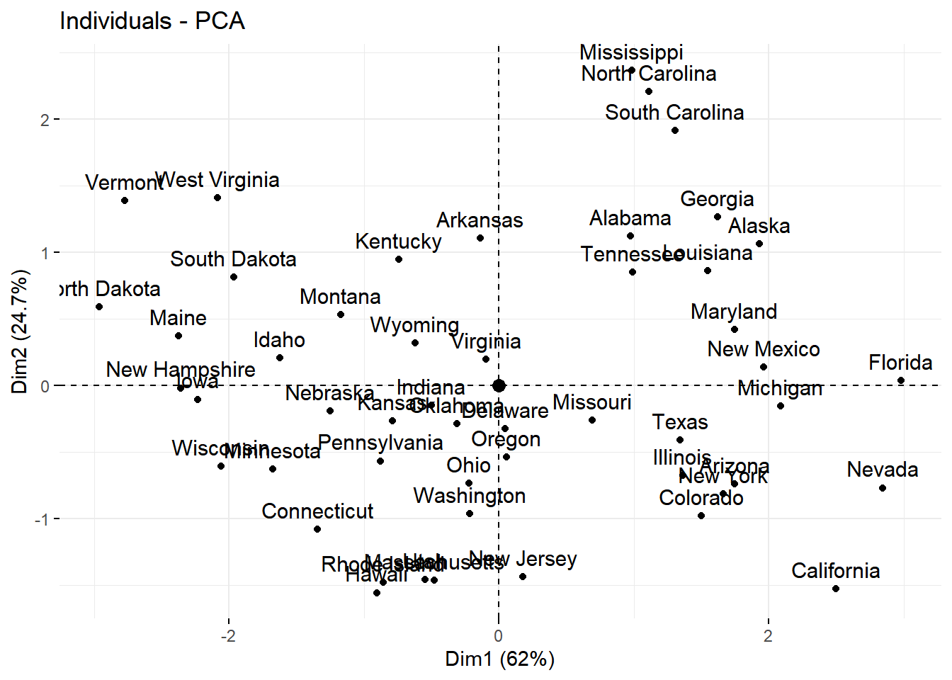
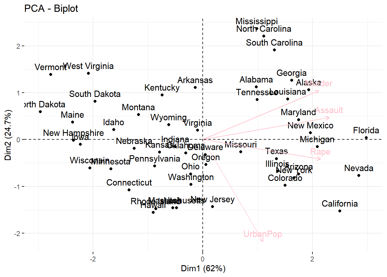
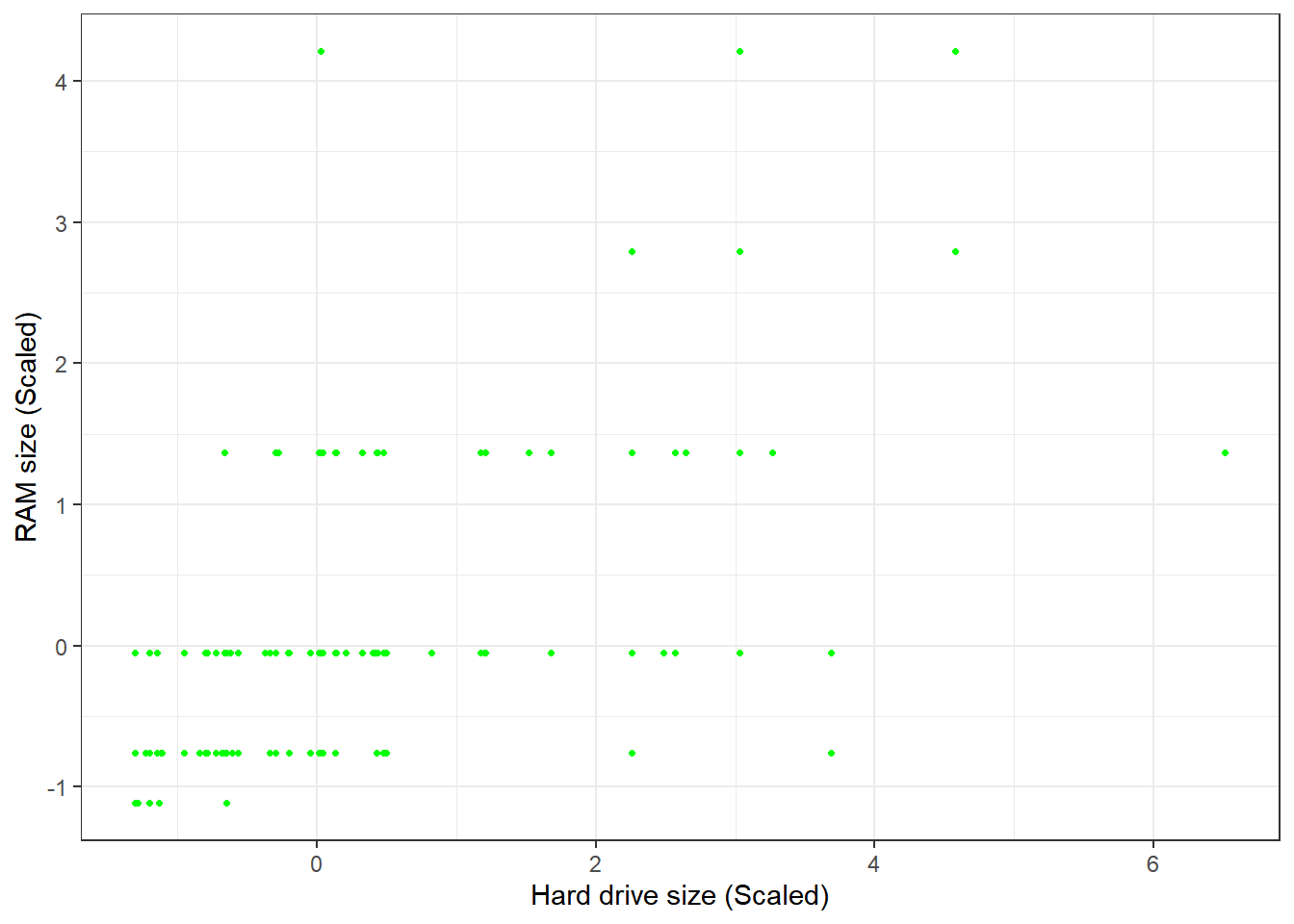
## Gentle Machine Learning## Principal Component Analysis# Dataset: USArrests is the sample dataset used in # McNeil, D. R. (1977) Interactive Data Analysis. New York: Wiley.# Murder numeric Murder arrests (per 100,000)# Assault numeric Assault arrests (per 100,000)# UrbanPop numeric Percent urban population# Rape numeric Rape arrests (per 100,000)# For each of the fifty states in the United States, the dataset contains the number # of arrests per 100,000 residents for each of three crimes: Assault, Murder, and Rape. # UrbanPop is the percent of the population in each state living in urban areas.library(datasets)library(ISLR)arrest = USArrestsstates=row.names(USArrests)names(USArrests)
[1] "Murder" "Assault" "UrbanPop" "Rape"
# Get means and variances of variablesapply(USArrests, 2, mean)
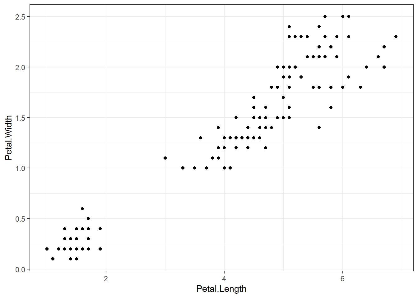
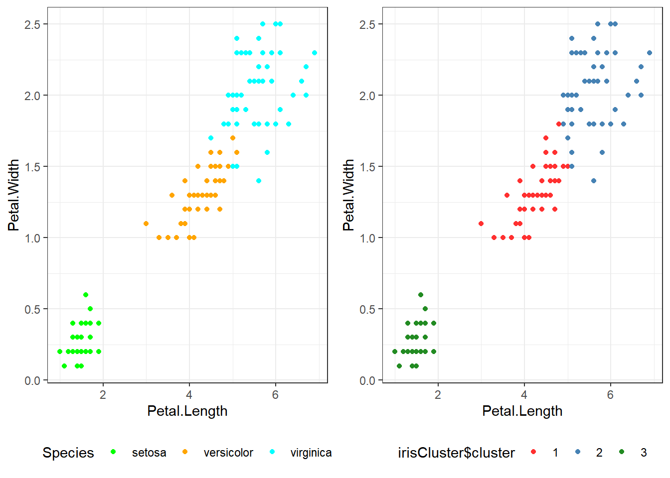
## Iris example# Without grouping by speciesggplot(iris, aes(Petal.Length, Petal.Width)) +geom_point() +theme_bw() +scale_color_manual(values=c("green","magenta","cyan"))
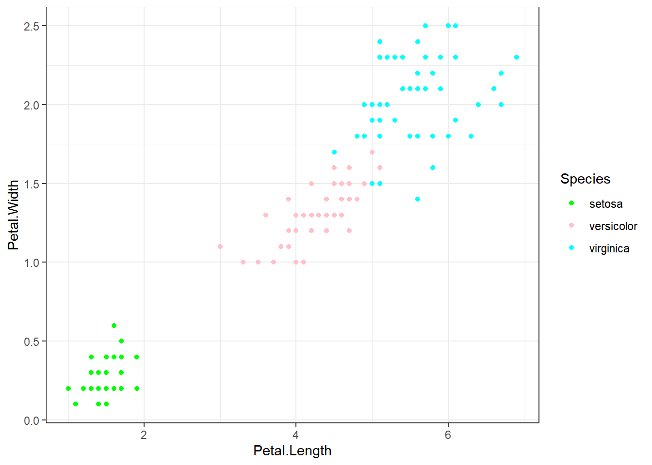
# With grouping by speciesggplot(iris, aes(Petal.Length, Petal.Width, color = Species)) +geom_point() +theme_bw() +scale_color_manual(values=c("green","pink","cyan"))
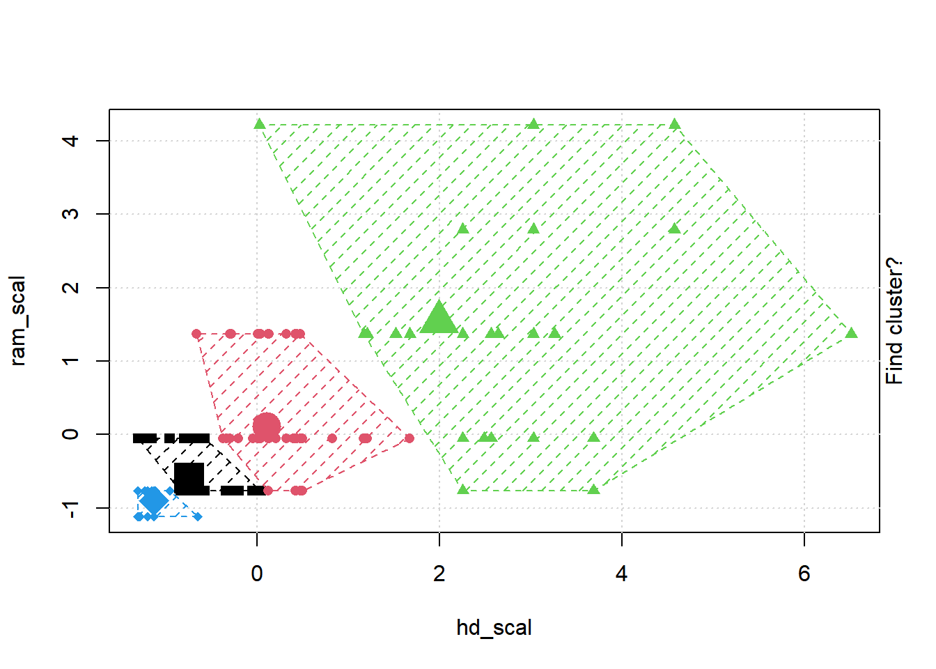
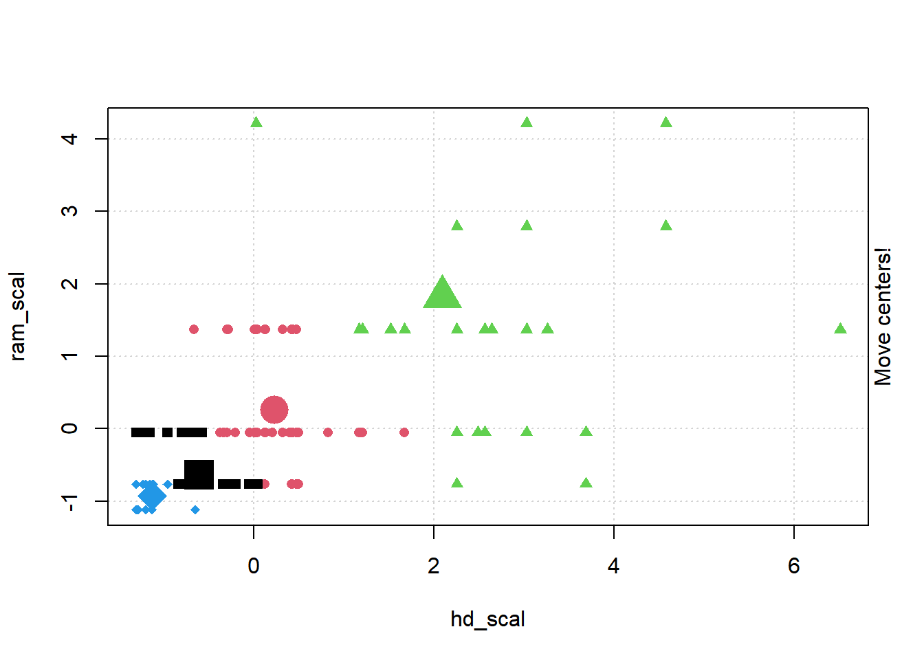
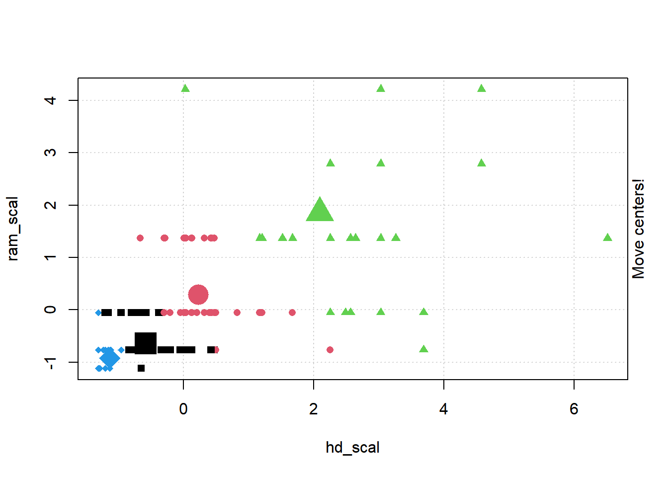
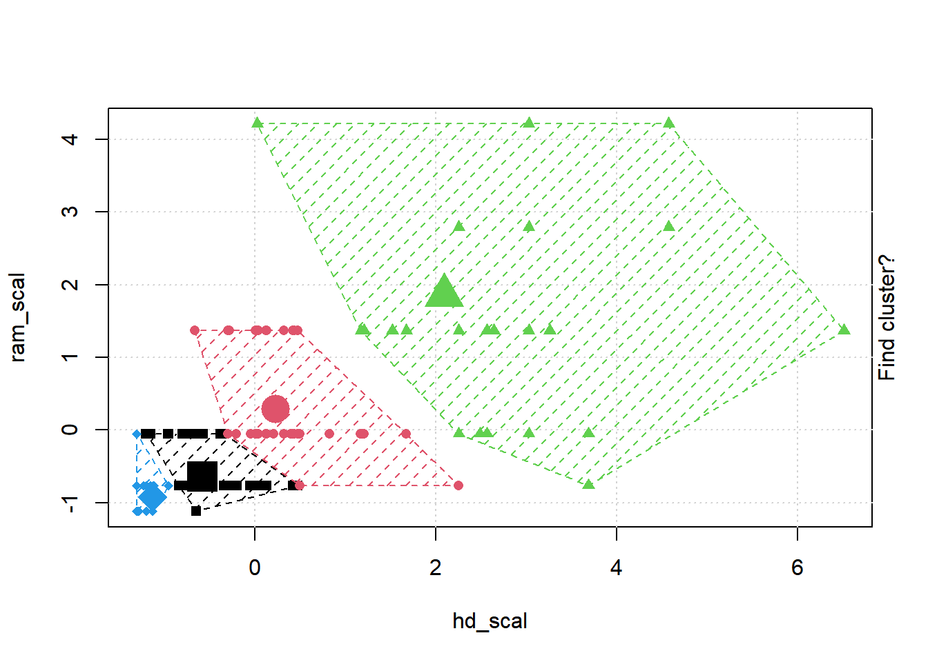
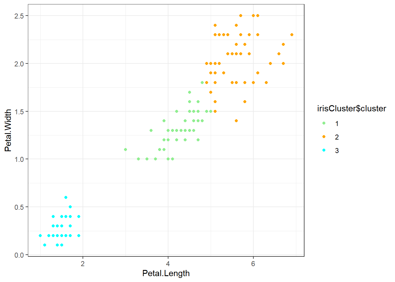
# Check k-means clusters## Starting with three clusters and 20 initial configurationsset.seed(20)irisCluster <-kmeans(iris[, 3:4], 3, nstart =20)irisCluster
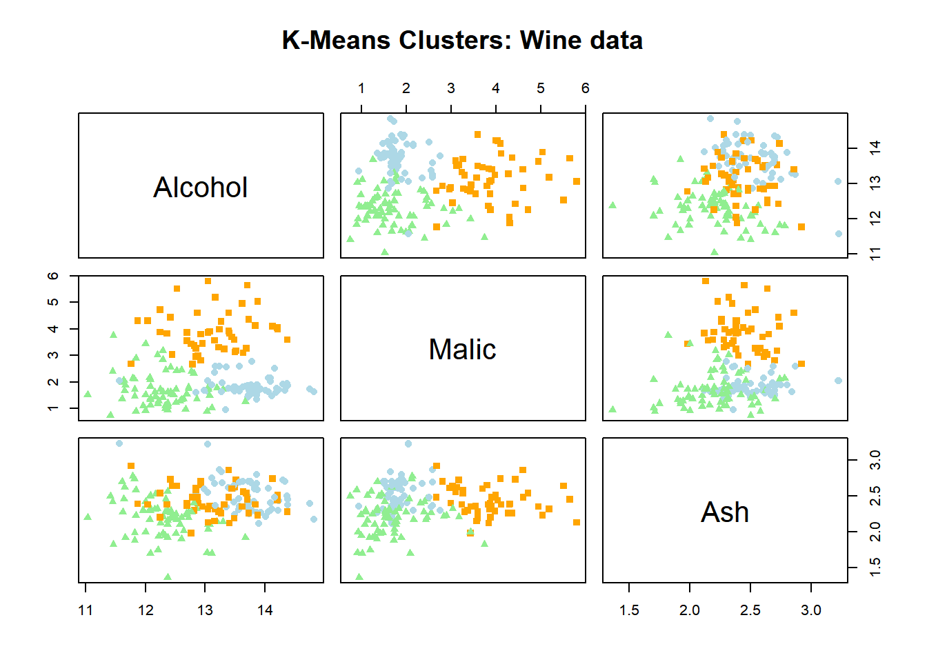
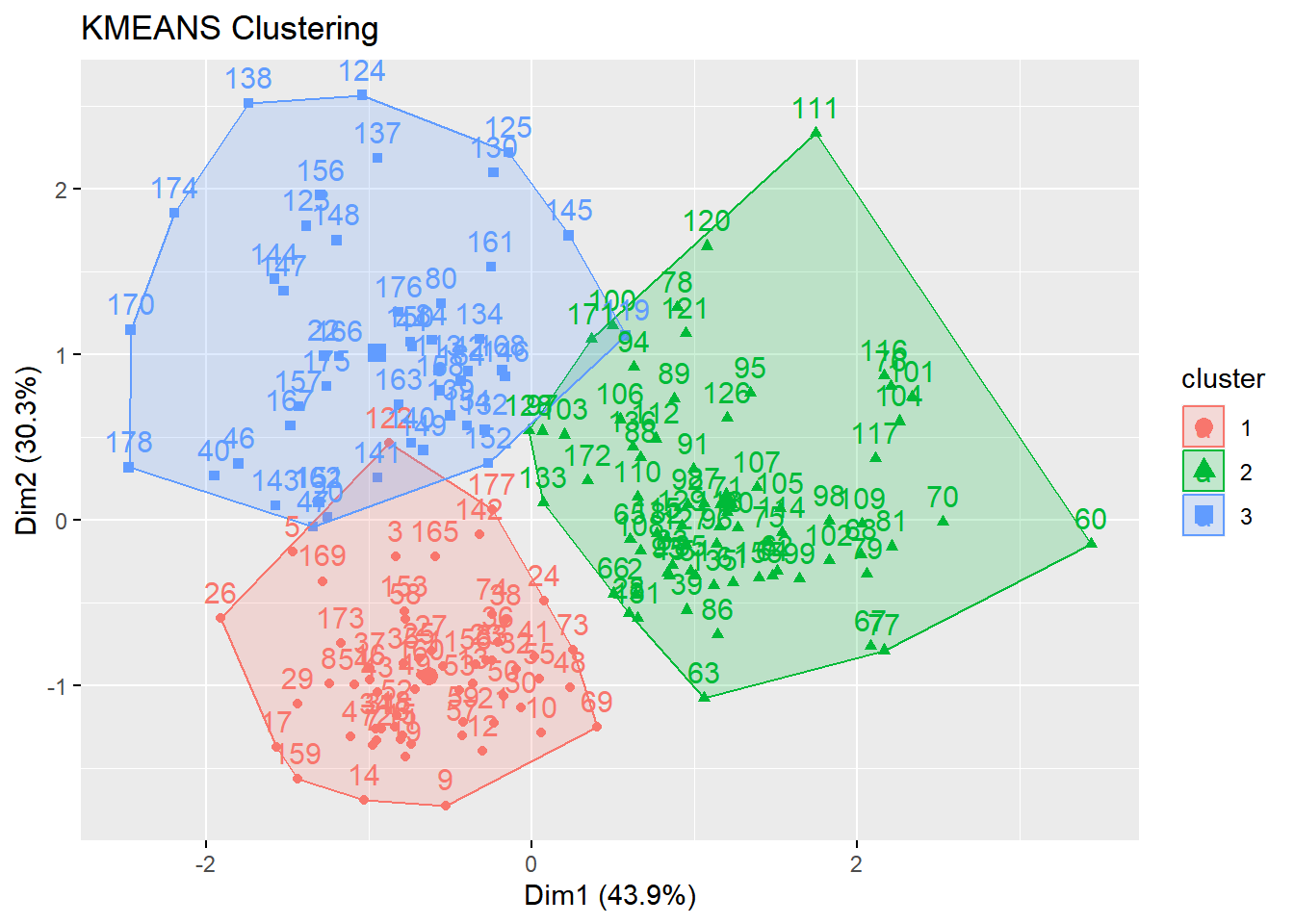
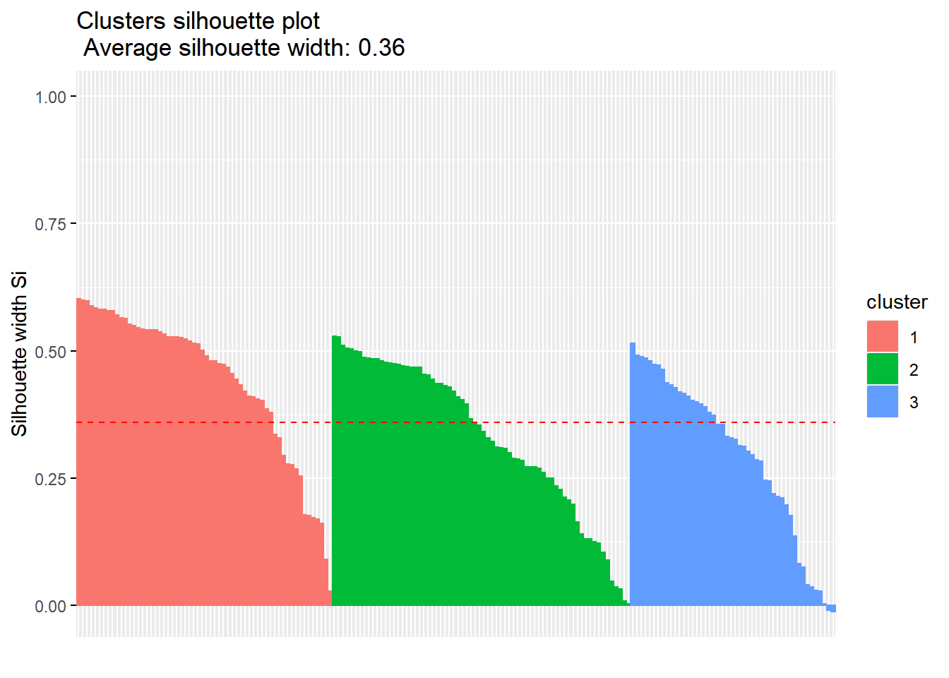
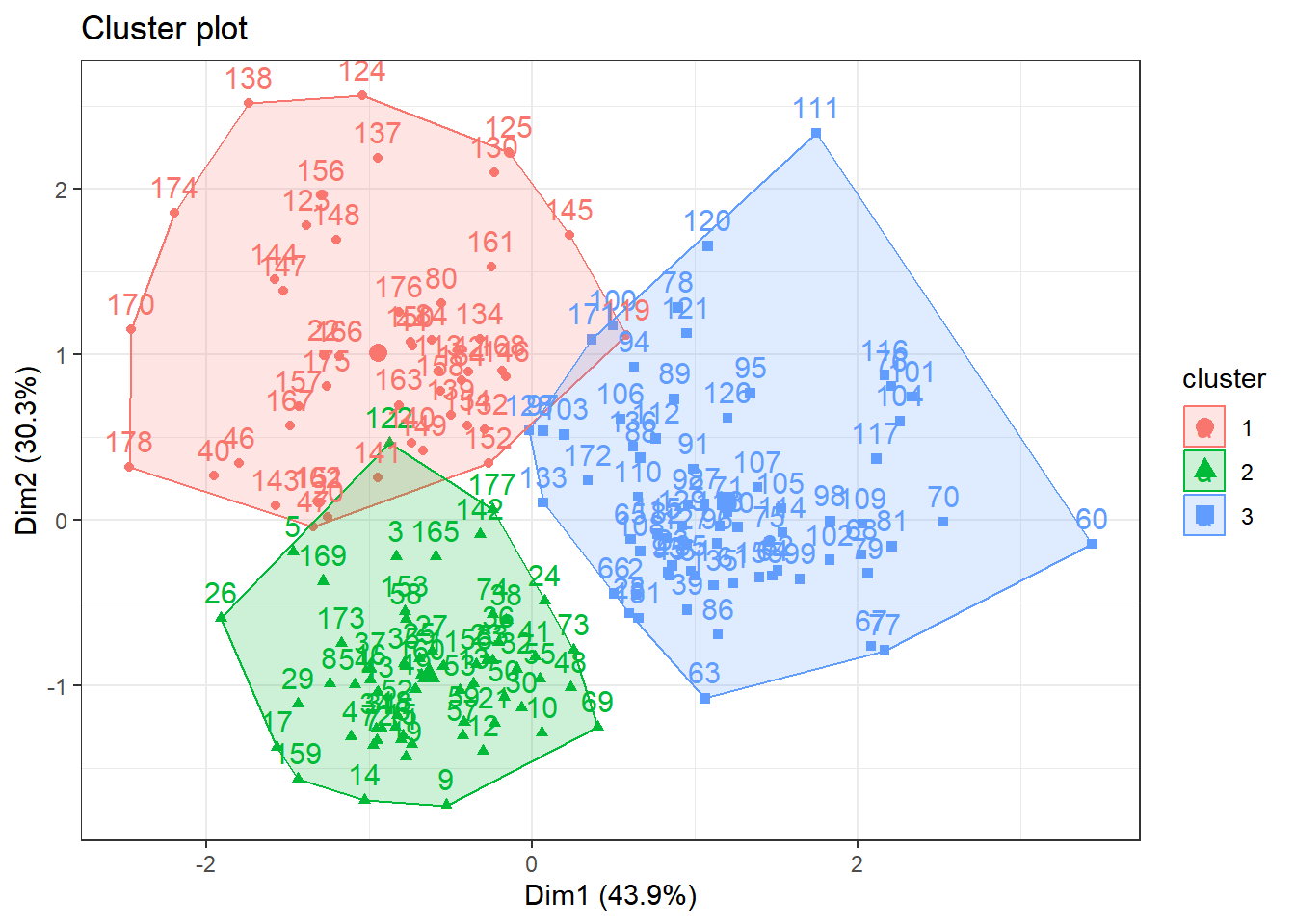
## Wine example# The wine dataset contains the results of a chemical analysis of wines # grown in a specific area of Italy. Three types of wine are represented in the 178 samples, with the results of 13 chemical analyses recorded for each sample. # Variables used in this example: Alcohol, Malic: Malic acid, Ash# Source: http://archive.ics.uci.edu/ml/datasets/Wine# Import wine datasetlibrary(readr)wine <-read_csv("https://raw.githubusercontent.com/datageneration/gentlemachinelearning/master/data/wine.csv")## Choose and scale variableswine_subset <-scale(wine[ , c(2:4)])## Create cluster using k-means, k = 3, with 25 initial configurationswine_cluster <-kmeans(wine_subset, centers =3,iter.max =10,nstart =25)wine_cluster
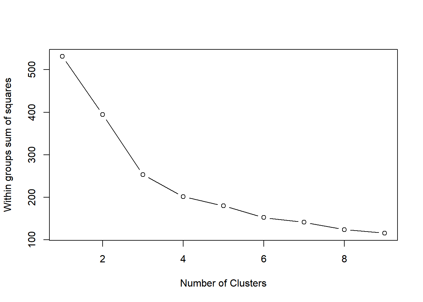
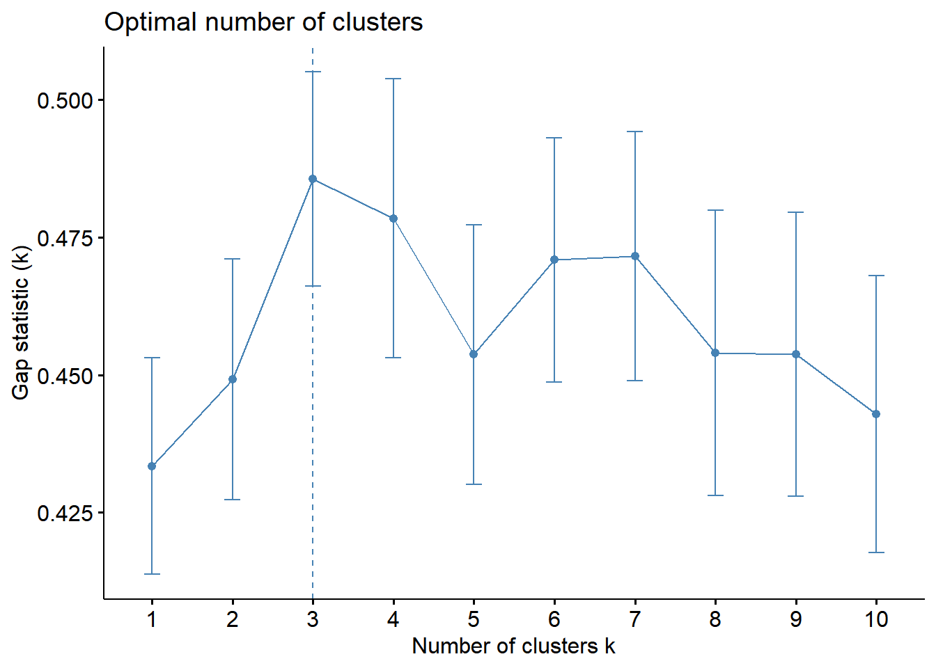
# Create a function to compute and plot total within-cluster sum of square (within-ness)wssplot <-function(data, nc=15, seed=1234){ wss <- (nrow(data)-1)*sum(apply(data,2,var))for (i in2:nc){set.seed(seed) wss[i] <-sum(kmeans(data, centers=i)$withinss)}plot(1:nc, wss, type="b", xlab="Number of Clusters",ylab="Within groups sum of squares")}# plotting values for each cluster starting from 1 to 9wssplot(wine_subset, nc =9)
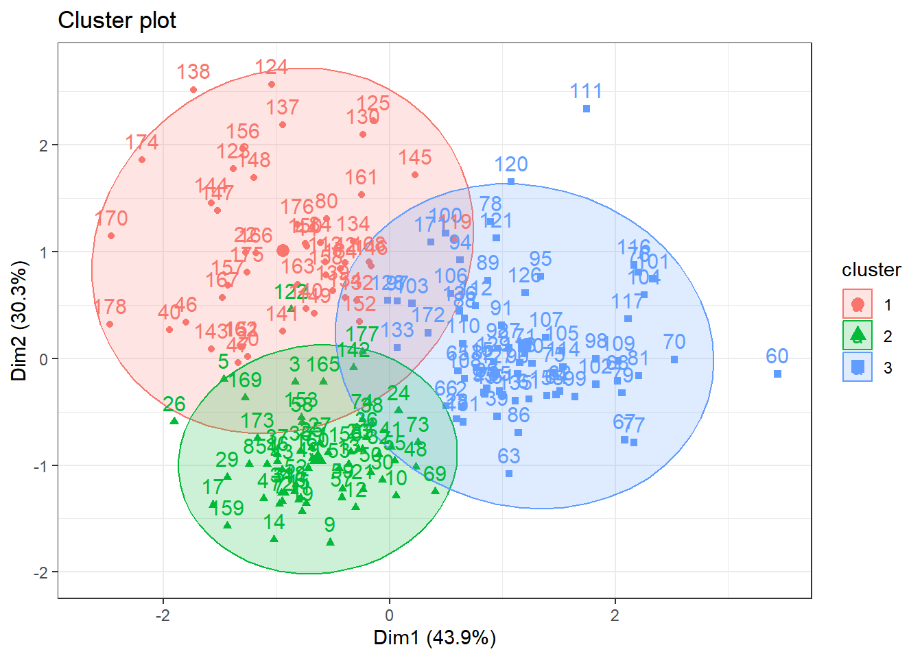
fviz_cluster(wine_cluster, data = wine_subset) +theme_bw() +theme(text =element_text(family="Georgia"))
fviz_cluster(wine_cluster, data = wine_subset, ellipse.type ="norm") +theme_bw() +theme(text =element_text(family="Georgia"))
3. Hierarchical Clustering
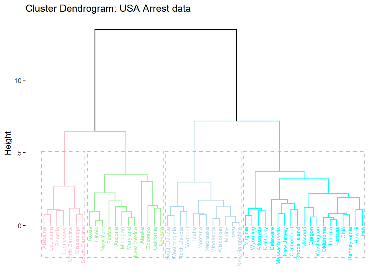
## Hierarchical Clustering## Dataset: USArrests# install.packages("cluster")arrest.hc <- USArrests %>%scale() %>%# Scale all variablesdist(method ="euclidean") %>%# Euclidean distance for dissimilarity hclust(method ="ward.D2") # Compute hierarchical clustering# Generate dendrogram using factoextra packagefviz_dend(arrest.hc, k =4, # Four groupscex =0.5, k_colors =c("pink","lightgreen","lightblue", "cyan"),color_labels_by_k =TRUE, # color labels by groupsrect =TRUE, # Add rectangle (cluster) around groups,main ="Cluster Dendrogram: USA Arrest data") +theme(text =element_text(family="Georgia"))
#Answer
Principal Component Analysis (PCA) and clustering methods play different roles in data analysis.
PCA aims to reduce dimensionality by transforming original variables into orthogonal variables known as principal components.
On the other hand, clustering methods aim to reveal natural groupings within the data by partitioning it into clusters of similar data points using similarity or distance metrics.
While PCA condenses information, clustering methods help in identifying inherent structures or patterns by grouping data points with common characteristics.
#References
References
James, Gareth, Daniela Witten, Trevor Hastie, and Robert Tibshirani. 2013 An introduction to statistical learning. Vol. 112. New York: Springer.