# Load necessary libraries in a single line
library(haven) # For reading Stata data files

Warning: package 'haven' was built under R version 4.3.2

library(MASS)  # For ordinal logistic regression

Warning: package 'MASS' was built under R version 4.3.2

library(vcd) # For categorical data

Warning: package 'vcd' was built under R version 4.3.2

Loading required package: grid

library(ggplot2)
library(tidyr)
library(grid)
library(dplyr)


Attaching package: 'dplyr'

The following object is masked from 'package:MASS':

    select

The following objects are masked from 'package:stats':

    filter, lag

The following objects are masked from 'package:base':

    intersect, setdiff, setequal, union

# Read the dataset and define variables in fewer lines
TEDS_2016 <- read_stata("https://github.com/datageneration/home/blob/master/DataProgramming/data/TEDS_2016.dta?raw=true")
variables <- c("Tondu", "age", "income", "edu")

# Loop for missing values, factor conversion, and checking levels consolidated
for (var in variables) {
  missing_count <- sum(is.na(TEDS_2016[[var]]))
  cat(var, "has", missing_count, "missing values\n")
}

Tondu has 0 missing values
age has 0 missing values
income has 0 missing values
edu has 10 missing values

TEDS_2016 <- within(TEDS_2016, {
  age_factor <- cut(age, breaks = c(19, 29, 39, 49, 59, Inf), labels = c("20-29",
                                                                         "30-39",
                                                                         "40-49",
                                                                         "50-59",
                                                                         "Above 60"), right = TRUE)
  income_factor <- factor(income, levels = c("1", "2", "3", "4", "5", "6", "7", "8", "9", "10", "5.5"),
                          labels = c("Under 28,000",
                                     "28,001-39,000",
                                     "39,001-49,000",
                                     "49,001-59,000",
                                     "59,001-69,000",
                                     "69,001-80,000",
                                     "80,001-93,000",
                                     "93,001-111,000",
                                     "111,001-141,000",
                                     "Over 141,001",
                                     "Other/Unknown"))
  edu_factor <- factor(edu, levels = c(1, 2, 3, 4, 5, 9), labels = c("Below elementary school",
                                                                     "Junior high school",
                                                                     "Senior high school",
                                                                     "College",
                                                                     "Above university",
                                                                     "Nonresponse"))
  Tondu_factor <- factor(Tondu, levels = c(1, 2, 3, 4, 5, 6, 9), labels = c("Immediate unification",
                                                                            "Maintain the status quo, move toward unification",
                                                                            "Maintain the status quo, decide either unification or independence",
                                                                            "Maintain the status quo forever",
                                                                            "Maintain the status quo, move toward independence",
                                                                            "Immediate independence",
                                                                            "Nonresponse"))
})



# Binary and numerical columns imputation consolidated
binary_columns <- sapply(TEDS_2016, function(x) all(x %in% c(0, 1, NA)))
TEDS_2016[, binary_columns] <- lapply(TEDS_2016[, binary_columns], function(x) {
  factor(x, levels = c(0, 1))
})
numerical_columns <- sapply(TEDS_2016, is.numeric) & !binary_columns
TEDS_2016[, numerical_columns] <- lapply(TEDS_2016[, numerical_columns], function(x) {
  ifelse(is.na(x), mean(x, na.rm = TRUE), x)
})
categorical_columns <- sapply(TEDS_2016, is.factor)
TEDS_2016[, categorical_columns] <- lapply(TEDS_2016[, categorical_columns], function(x) {
  mode_value <- names(which.max(table(x)))
  factor(ifelse(is.na(x), mode_value, x), levels = levels(x))
})

regplot <- function(x, y, title, xlab = "X", ylab = "Y") {
  fit <- lm(y ~ x)
  plot(x, y, main = paste("Regression Fit Plot", title), xlab = xlab, ylab = ylab, pch = 20)
  abline(fit, col = "green")
}

# Regression plot function usage consolidated
TEDS_2016$Tondu_numeric <- as.numeric(as.character(TEDS_2016$Tondu))
regplot(TEDS_2016$age, TEDS_2016$Tondu_numeric, "Age vs. Tondu", xlab = "Age", ylab = "Tondu Response")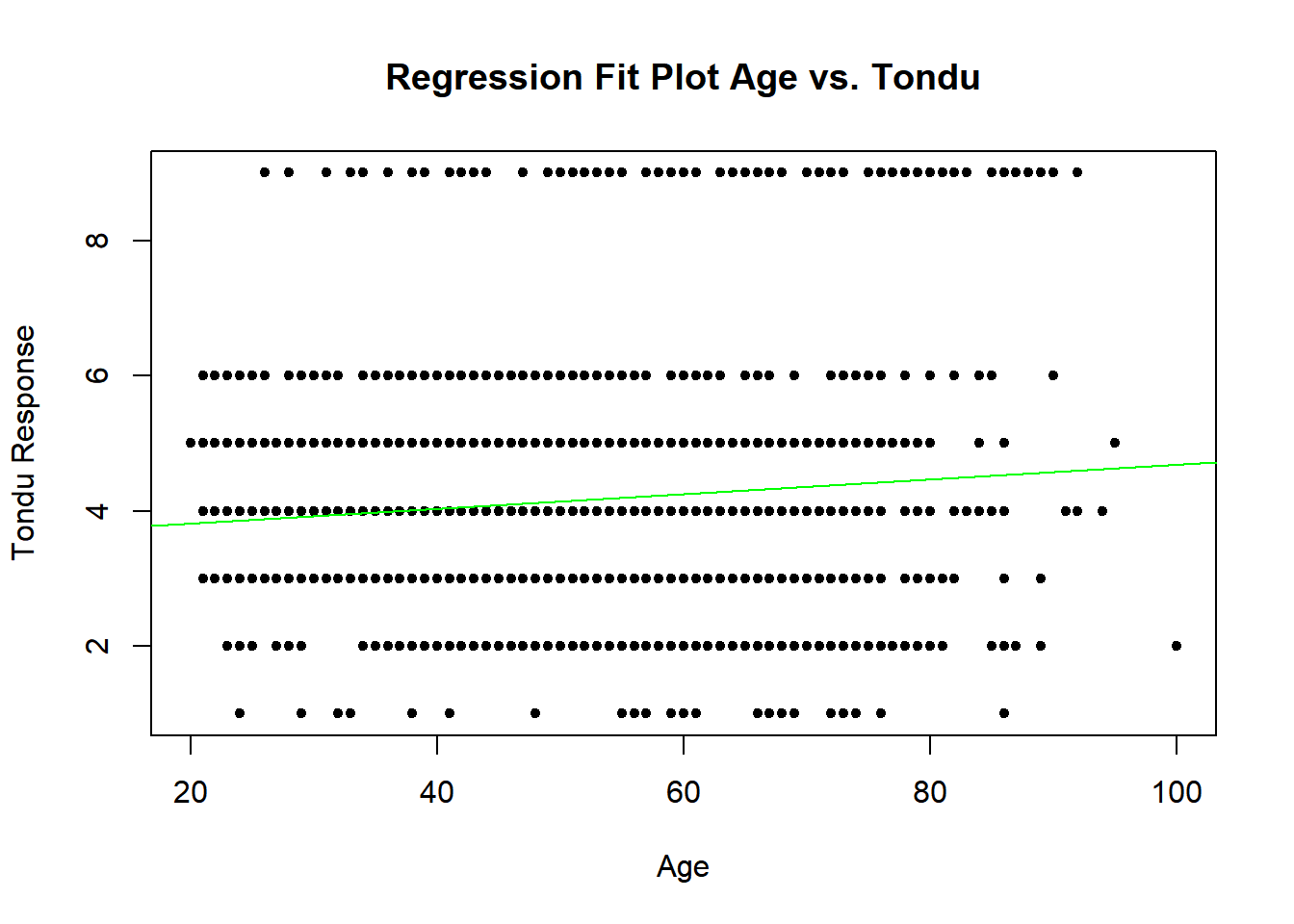

regplot(TEDS_2016$edu, TEDS_2016$Tondu_numeric, "Education vs. Tondu", xlab = "Education Level", ylab = "Tondu Response")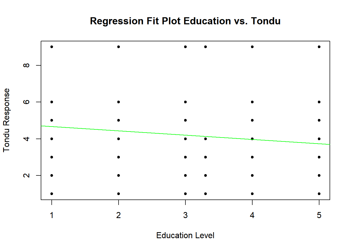

regplot(TEDS_2016$income, TEDS_2016$Tondu_numeric, "Income vs. Tondu", xlab = "Income Category", ylab = "Tondu Response")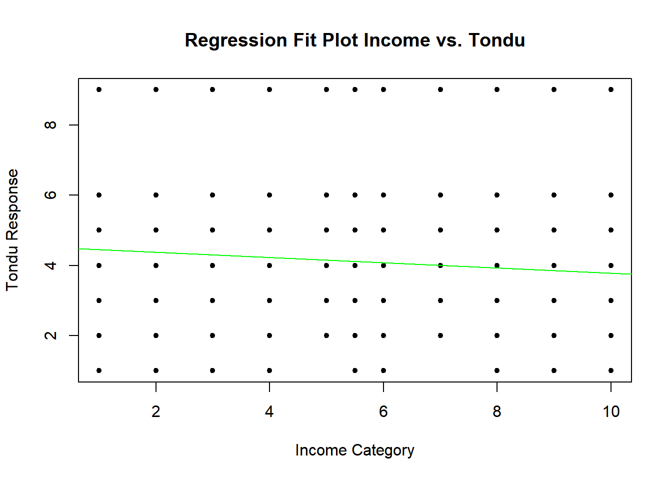

# Ordinal logistic regression and plotting consolidated

pred_data_age <- data.frame(age_factor = levels(TEDS_2016$age_factor))

Answer

Problem: The regression plot seems to lack significance, likely because the Tondu variable is divided into 7 categories.

Suggestion: Given the categorical nature of the data, linear regression may not be the best fit. Instead, logistic regression could be a more suitable choice.